Advanced Next-Generation Workflows in PubChemR

This vignette has two layers.

The first layer is researcher-facing: a concrete compound-triage workflow that answers the question “what can I actually do with PubChemR?”.

The second layer is systems-facing: the transport, caching, async, batching, and typed-result machinery that makes those workflows reproducible and robust.

It is designed to be:

Offline-first and reproducible by default.
Structured from basic to advanced usage.
Practical for production pipelines.
Explicit about object contracts, failures, and edge cases.

How to use this guide:

Read each section in order on first pass; later sections depend on earlier transport and object-contract concepts.
If you are primarily a researcher, start with the scientific workflow below and then return to the architecture sections only as needed.
If you are building pipelines or package integrations, the later sections document the nextgen contracts in detail.

How to read each section:

Each major section is written to answer four questions: what problem this part of the package solves, what object or table it returns, how to tell if the result is usable, and what the next step usually is.
Each subsection follows the same pattern: Purpose tells you when to use a function, the Minimal example shows the smallest valid call, the Typical example shows a realistic workflow call, the Advanced example shows how the function behaves in robust pipeline code, and Interpretation explains how to read the returned object.
When an example returns a typed object rather than a plain table, the first things to inspect are success, error, pending, from_cache, and request metadata from request_args().
When an example returns a table, focus first on the row meaning, the key identifier columns (CID, SID, AID), and whether the output is already suitable for joining, plotting, or modeling.

Research-First Workflow

This section answers the practical question a typical PubChemR user starts with:

“Given a known compound, how do I triage related compounds by properties and assay activity?”

The example below uses an aspirin-like seed structure. In live mode it can query PubChem similarity results; in offline mode it falls back to exported deterministic example data so the workflow still runs end-to-end.

library(PubChemR)
library(dplyr)
#> 
#> Attaching package: 'dplyr'
#> The following objects are masked from 'package:stats':
#> 
#>     filter, lag
#> The following objects are masked from 'package:base':
#> 
#>     intersect, setdiff, setequal, union
library(tibble)

run_live <- identical(Sys.getenv("PUBCHEMR_RUN_LIVE"), "true")

`%||%` <- function(x, y) if (is.null(x)) y else x

safe_call <- function(expr) {
  tryCatch(
    expr,
    error = function(e) structure(list(message = conditionMessage(e)), class = "pc_error")
  )
}

summarize_any <- function(x) {
  if (inherits(x, "pc_error")) {
    return(tibble(ok = FALSE, class = "pc_error", note = x$message, rows = NA_integer_, cols = NA_integer_))
  }

  if (inherits(x, "PubChemResult")) {
    return(tibble(
      ok = isTRUE(x$success),
      class = class(x)[1],
      note = if (isTRUE(x$success)) "success" else (x$error$code %||% "error"),
      rows = nrow(as_tibble(x)),
      cols = ncol(as_tibble(x))
    ))
  }

  if (inherits(x, "PubChemAsyncQuery")) {
    return(tibble(ok = TRUE, class = class(x)[1], note = "async query object", rows = NA_integer_, cols = NA_integer_))
  }

  if (is.data.frame(x)) {
    return(tibble(ok = TRUE, class = class(x)[1], note = "tabular output", rows = nrow(x), cols = ncol(x)))
  }

  tibble(ok = TRUE, class = class(x)[1], note = "non-tabular output", rows = NA_integer_, cols = NA_integer_)
}

Use Case

Goal:

Start from a known analgesic scaffold.
Resolve or reuse a small candidate set.
Retrieve or reuse physicochemical properties.
Attach assay activity evidence.
Filter to compounds that look drug-like and show any evidence of activity.

research_seed_smiles <- "CC(=O)OC1=CC=CC=C1C(=O)O"

assay_payload <- pc_example_assaysummary_payload()
feature_tbl_synthetic <- pc_example_feature_table() %>%
  mutate(
    CanonicalSMILES = c(
      "CC(=O)OC1=CC=CC=C1C(=O)O",
      "CC(C)CC1=CC=C(C=C1)C(C)C(=O)O",
      "CN1C=NC2=C1C(=O)N(C(=O)N2)C"
    )
  )

research_similarity <- if (run_live) {
  pc_similarity_search(
    identifier = research_seed_smiles,
    namespace = "smiles",
    threshold = 90,
    max_records = 25,
    cache = TRUE
  )
} else {
  pc_similarity_search(
    identifier = research_seed_smiles,
    namespace = "smiles",
    threshold = 90,
    max_records = 25,
    cache = TRUE,
    offline = TRUE
  )
}

research_cids <- if (inherits(research_similarity, "PubChemResult") && isTRUE(research_similarity$success)) {
  as_tibble(research_similarity) %>%
    filter(!is.na(CID)) %>%
    transmute(CID = as.character(CID)) %>%
    distinct()
} else {
  feature_tbl_synthetic %>%
    transmute(CID)
}

research_features_try <- pc_feature_table(
  identifier = research_cids$CID,
  properties = c("MolecularWeight", "XLogP", "TPSA", "HBondDonorCount", "HBondAcceptorCount"),
  namespace = "cid",
  cache = TRUE,
  offline = !run_live,
  error_mode = "result"
)

research_features <- if (inherits(research_features_try, "PubChemResult")) {
  feature_tbl_synthetic
} else {
  research_features_try %>%
    mutate(CID = as.character(CID))
}

research_assay_long <- pc_assay_activity_long(
  x = assay_payload,
  add_outcome_value = TRUE
)

research_activity_summary <- research_assay_long %>%
  group_by(CID) %>%
  summarise(
    n_assays = n(),
    outcomes = paste(sort(unique(ActivityOutcome)), collapse = ", "),
    any_active = any(ActivityOutcomeValue == 1, na.rm = TRUE),
    median_activity_uM = if (all(is.na(ActivityValue_uM))) NA_real_ else median(ActivityValue_uM, na.rm = TRUE),
    .groups = "drop"
  )

research_triage <- research_features %>%
  left_join(research_activity_summary, by = "CID") %>%
  mutate(
    n_assays = ifelse(is.na(n_assays), 0L, as.integer(n_assays)),
    any_active = ifelse(is.na(any_active), FALSE, any_active),
    outcomes = ifelse(is.na(outcomes), "No assay evidence", outcomes),
    passes_rule_of_five_like =
      MolecularWeight <= 500 &
        XLogP <= 5 &
        HBondDonorCount <= 5 &
        HBondAcceptorCount <= 10,
    activity_bucket = case_when(
      any_active ~ "Any Active",
      n_assays > 0 ~ "Assayed, no active hit",
      TRUE ~ "No assay evidence in fixture"
    )
  ) %>%
  arrange(desc(any_active), desc(passes_rule_of_five_like), MolecularWeight)

research_triage %>%
  select(CID, MolecularWeight, XLogP, TPSA, n_assays, any_active, passes_rule_of_five_like, activity_bucket)
#> # A tibble: 3 × 8
#>   CID   MolecularWeight XLogP  TPSA n_assays any_active passes_rule_of_five_like
#>   <chr>           <dbl> <dbl> <dbl>    <int> <lgl>      <lgl>                   
#> 1 2244             180.   1.2  63.6        2 TRUE       TRUE                    
#> 2 5957             194.   0.1  86.6        0 FALSE      TRUE                    
#> 3 3672             206.   3.5  37.3        1 FALSE      TRUE                    
#> # ℹ 1 more variable: activity_bucket <chr>

What this shows:

PubChemR can support a familiar medicinal-chemistry screening pattern: seed compound -> candidate set -> properties -> assay evidence -> triage.
The same code path can be live or deterministic depending on run_live.
The nextgen layer is useful here because data acquisition can fail while the workflow still remains explicit and reproducible.

Filter and Rank

research_ranked <- research_triage %>%
  filter(passes_rule_of_five_like) %>%
  mutate(
    potency_score = ifelse(is.na(median_activity_uM), 0, 1 / (1 + median_activity_uM)),
    rank_score =
      2 * as.numeric(any_active) +
        potency_score +
        0.10 * n_assays -
        abs(XLogP - 2.5) / 5
  ) %>%
  arrange(desc(rank_score), MolecularWeight) %>%
  mutate(rank = row_number())

list(
  total_candidates = nrow(research_triage),
  druglike_candidates = nrow(research_ranked),
  top_candidates = research_ranked %>%
    select(rank, CID, MolecularWeight, XLogP, n_assays, any_active, median_activity_uM, rank_score)
)
#> $total_candidates
#> [1] 3
#> 
#> $druglike_candidates
#> [1] 3
#> 
#> $top_candidates
#> # A tibble: 3 × 8
#>    rank CID   MolecularWeight XLogP n_assays any_active median_activity_uM
#>   <int> <chr>           <dbl> <dbl>    <int> <lgl>                   <dbl>
#> 1     1 2244             180.   1.2        2 TRUE                      1.2
#> 2     2 3672             206.   3.5        1 FALSE                    12.5
#> 3     3 5957             194.   0.1        0 FALSE                    NA  
#> # ℹ 1 more variable: rank_score <dbl>

Interpretation:

The workflow now completes the usual screening loop: retrieve, filter, summarize activity, then rank candidates.
The ranking formula is intentionally simple and transparent; it is a vignette-level triage score, not a production QSAR model.

Pipeline Diagram

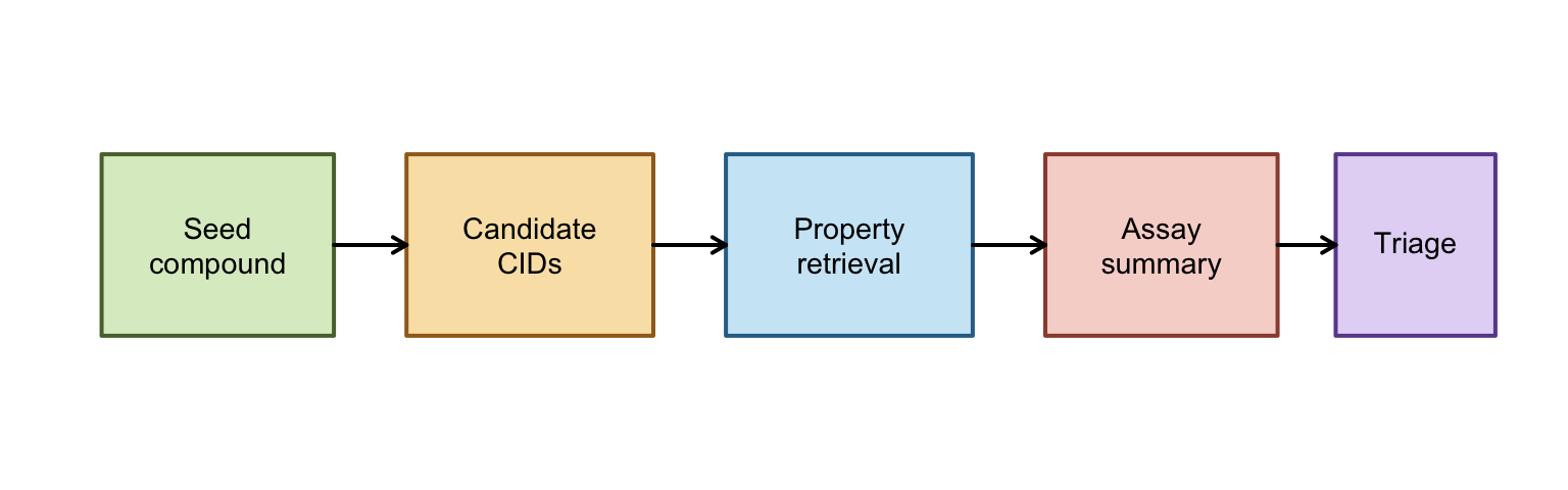
Interpretation:

This diagram is the mental model for the rest of the vignette: each box is a stage where PubChemR changes the shape of the data, not just retrieves it.
The early boxes are retrieval-focused, the middle boxes are normalization and summarization, and the final box is where scientific judgment enters through filtering and ranking.
If a later section feels abstract, map it back to one box here and ask what that stage must return for the next stage to work.

Quick Plots

op <- par(mfrow = c(2, 2), mar = c(4, 4, 2, 1))

hist(
  research_triage$MolecularWeight,
  main = "Candidate Molecular Weight",
  xlab = "MolecularWeight",
  col = "#CDE8F6",
  border = "white"
)

barplot(
  table(research_assay_long$ActivityOutcome),
  main = "Activity Outcome Counts",
  ylab = "Count",
  las = 2,
  col = c("#DCECC9", "#F9E3B4", "#F6D6D0")
)

plot(
  research_triage$XLogP,
  research_triage$MolecularWeight,
  pch = 19,
  col = ifelse(research_triage$any_active, "#58713A", "#9B4D3A"),
  xlab = "XLogP",
  ylab = "MolecularWeight",
  main = "Property Space by Activity"
)
text(
  research_triage$XLogP,
  research_triage$MolecularWeight,
  labels = research_triage$CID,
  pos = 3,
  cex = 0.8
)

barplot(
  research_ranked$rank_score,
  names.arg = research_ranked$CID,
  main = "Ranked Candidate Scores",
  ylab = "rank_score",
  col = "#E4D8F5",
  las = 2
)


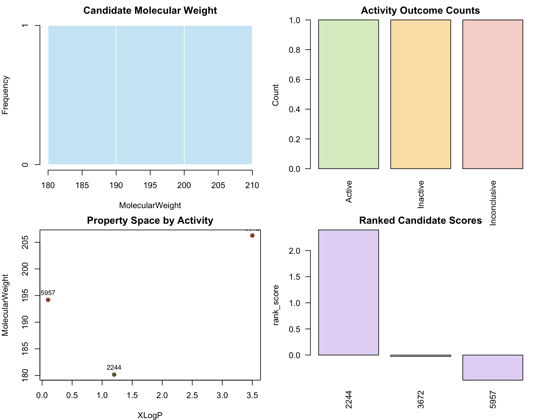
par(op)

Interpretation:

The histogram answers whether the candidate set sits in a plausible molecular weight range for small-molecule screening.
The activity bar chart answers whether the assay evidence is informative or mostly empty/inconclusive.
The property-space scatter plot answers whether active and inactive compounds occupy obviously different regions of simple descriptor space.
The ranked-score plot answers whether the workflow produces a usable ordering rather than only a raw collection of records.

Why It Matters

The rest of this vignette explains the machinery behind the workflow above:

how requests are represented as typed objects,
how cache/offline policies are controlled,
how async and batch workflows are recovered safely,
and how the analysis helpers connect retrieval to model-ready data.

Roadmap

The next-generation API in PubChemR centers around typed result objects, policy-controlled transport, orchestration helpers, and analysis-layer tools.

Read this section as a map, not as something you need to memorize. Its purpose is to show where each function family belongs in a real workflow and why the same package contains both scientific helpers and infrastructure helpers.

nextgen_function_map <- tibble(
  family = c(
    rep("Transport", 6),
    rep("Wrappers", 7),
    rep("Async", 3),
    rep("Batch/Benchmark", 4),
    rep("Analysis", 10),
    rep("Helpers", 6)
  ),
  function_name = c(
    "pc_profile", "pc_config", "pc_request", "pc_response", "pc_cache_info/pc_cache_clear", "pc_capabilities",
    "pc_compound", "pc_substance", "pc_assay", "pc_property", "pc_identifier_map", "pc_similarity_search", "pc_sdq_bioactivity",
    "pc_submit", "pc_poll", "pc_collect",
    "pc_batch", "pc_resume_batch", "pc_benchmark", "pc_benchmark_harness",
    "pc_assay_activity_long", "pc_activity_outcome_map", "pc_activity_matrix", "pc_cross_domain_join",
    "pc_feature_table", "pc_model_matrix", "pc_export_model_data", "pc_to_rcdk", "pc_to_chemminer", "pc_lifecycle_policy",
    "pc_example_assaysummary_payload", "pc_example_feature_table", "as_tibble", "request_args", "has_hits", "retrieve"
  )
)

nextgen_function_map
#> # A tibble: 36 × 2
#>    family    function_name               
#>    <chr>     <chr>                       
#>  1 Transport pc_profile                  
#>  2 Transport pc_config                   
#>  3 Transport pc_request                  
#>  4 Transport pc_response                 
#>  5 Transport pc_cache_info/pc_cache_clear
#>  6 Transport pc_capabilities             
#>  7 Wrappers  pc_compound                 
#>  8 Wrappers  pc_substance                
#>  9 Wrappers  pc_assay                    
#> 10 Wrappers  pc_property                 
#> # ℹ 26 more rows

What to expect:

This table is the roadmap for the rest of the vignette.
Every function listed above appears in runnable examples.
Live-network examples are explicitly guarded by run_live.
Exported deterministic fixtures are used wherever possible so examples stay stable offline.

How to interpret the roadmap:

Transport functions control how requests are made and how failures are represented.
Wrappers tell PubChem what kind of record you want.
Async and Batch/Benchmark functions become relevant when a workflow must scale or recover from interruptions.
Analysis functions turn retrieved data into tables, matrices, and exports a scientist can use directly.
Helpers are the glue for inspecting, standardizing, and reusing outputs.

Core object classes used throughout:

PubChemResult: typed transport result (success, data, error, metadata).
PubChemRecord/PubChemIdMap: specialized PubChemResult subclasses.
PubChemAsyncQuery: async container for submit/poll/collect workflows.
PubChemBatchResult: chunk-level execution summary and checkpoint metadata.
PubChemBenchmarkReport: scenario-level benchmark summary with pass/fail gates.
PubChemModelMatrix/PubChemSparseActivityMatrix: modeling-ready matrix wrappers.

Setup

A robust nextgen workflow starts with explicit transport policy and deterministic runtime settings.

Section contract:

Read this section before you trust any later example.
Inputs: runtime environment, cache location, and transport defaults.
Outputs: a known policy state and an auditable capability snapshot.
Interpret the outputs by asking: where is the cache, is live mode allowed, and do optional packages exist in this session.
Pitfalls: hidden global-state mutations and accidental live requests.
Performance note: stable cache policy is usually more important than raw request speed in iterative workflows.

cfg_before <- pc_config()
cfg_before
#> $rate_limit
#> [1] 5
#> 
#> $timeout
#> [1] 60
#> 
#> $retries
#> [1] 3
#> 
#> $pause_base
#> [1] 1
#> 
#> $pause_cap
#> [1] 8
#> 
#> $user_agent
#> [1] "PubChemR/3.0.0"
#> 
#> $cache_dir
#> [1] "/var/folders/dj/y28dp44x303ggfg6rg8n2v0h0000gn/T//RtmpHAl5DI/PubChemR_cache"
#> 
#> $cache_ttl
#> [1] 86400
#> 
#> $offline
#> [1] FALSE

pc_profile("default")
#> $rate_limit
#> [1] 5
#> 
#> $timeout
#> [1] 60
#> 
#> $retries
#> [1] 3
#> 
#> $pause_base
#> [1] 1
#> 
#> $pause_cap
#> [1] 8
#> 
#> $user_agent
#> [1] "PubChemR/3.0.0"
#> 
#> $cache_dir
#> [1] "/var/folders/dj/y28dp44x303ggfg6rg8n2v0h0000gn/T//RtmpHAl5DI/PubChemR_cache"
#> 
#> $cache_ttl
#> [1] 86400
#> 
#> $offline
#> [1] FALSE
cfg_after_profile <- pc_config()
cfg_after_profile[c("rate_limit", "timeout", "retries", "cache_ttl")]
#> $rate_limit
#> [1] 5
#> 
#> $timeout
#> [1] 60
#> 
#> $retries
#> [1] 3
#> 
#> $cache_ttl
#> [1] 86400

# Keep cache in a temp path during vignette execution.
work_cache <- file.path(tempdir(), "pubchemr-vignette-cache")
dir.create(work_cache, recursive = TRUE, showWarnings = FALSE)
pc_config(cache_dir = work_cache, offline = FALSE)
#> $rate_limit
#> [1] 5
#> 
#> $timeout
#> [1] 60
#> 
#> $retries
#> [1] 3
#> 
#> $pause_base
#> [1] 1
#> 
#> $pause_cap
#> [1] 8
#> 
#> $user_agent
#> [1] "PubChemR/3.0.0"
#> 
#> $cache_dir
#> [1] "/var/folders/dj/y28dp44x303ggfg6rg8n2v0h0000gn/T//RtmpjLjM6G/pubchemr-vignette-cache"
#> 
#> $cache_ttl
#> [1] 86400
#> 
#> $offline
#> [1] FALSE

pc_cache_clear(cache_dir = work_cache, memory = TRUE, disk = TRUE)
pc_cache_info(cache_dir = work_cache)
#> # A tibble: 1 × 4
#>   memory_entries disk_entries disk_size_bytes cache_dir                         
#>            <int>        <int>           <dbl> <chr>                             
#> 1              0            0               0 /var/folders/dj/y28dp44x303ggfg6r…

What to expect:

pc_profile() applies a baseline policy.
pc_config() confirms active runtime state.
Cache is isolated to tempdir() to avoid modifying user directories.

pc_capabilities(cache_dir = work_cache, check_network = FALSE)
#> # A tibble: 1 × 9
#>   live_enabled offline_mode cache_dir  cache_exists cache_writable optional_rcdk
#>   <lgl>        <lgl>        <chr>      <lgl>        <lgl>          <lgl>        
#> 1 TRUE         FALSE        /var/fold… TRUE         TRUE           FALSE        
#> # ℹ 3 more variables: optional_chemminer <lgl>, optional_matrix <lgl>,
#> #   network_reachable <lgl>

Interpretation:

pc_capabilities() gives a preflight summary for optional dependencies, cache writability, and offline/live mode.
Use this as an early diagnostic before long workflows or CI jobs.

Key pitfalls and notes:

rate_limit and cache_ttl are validated; invalid values fail early.
Use explicit cache directories in scripts for deterministic CI behavior.
Restore old config in project code when changing globals (pc_config(...)).

Core Contracts

The transport contract is the foundation for every other nextgen function.

If results feel abstract later in the vignette, come back here. This section defines what a “good” result looks like, what a controlled failure looks like, and why the package often returns objects rather than immediately returning a data frame.

Parsing Results

Purpose:

Normalize success/fault payloads into a stable structure (success, data, error, metadata).

Minimal example

ok_text <- '{"PropertyTable":{"Properties":[{"CID":2244,"MolecularWeight":180.16}]}}'
res_ok <- pc_response(
  ok_text,
  request = list(domain = "compound", namespace = "cid", identifier = 2244, operation = "property/MolecularWeight")
)

class(res_ok)
#> [1] "PubChemResult"
res_ok$success
#> [1] TRUE
as_tibble(res_ok)
#> # A tibble: 1 × 6
#>   success status from_cache pending   CID MolecularWeight
#>   <lgl>    <int> <lgl>      <lgl>   <dbl>           <dbl>
#> 1 TRUE        NA FALSE      FALSE    2244            180.

Interpretation:

success is TRUE and as_tibble() exposes payload content as a flat table.

Typical example

fault_text <- '{"Fault":{"Code":"PUGREST.BadRequest","Message":"Invalid request"}}'
res_fault <- pc_response(fault_text, request = list(domain = "compound"))

res_fault$success
#> [1] FALSE
res_fault$error$code
#> [1] "PUGREST.BadRequest"
res_fault$error$message
#> [1] "PUGREST.BadRequest" "Invalid request"

Interpretation:

Fault payloads remain structured; they do not crash the pipeline by default.
Downstream code can branch on success and error$code.

Advanced example

waiting_text <- '{"Waiting":{"ListKey":"example-listkey"}}'
res_wait <- pc_response(waiting_text, request = list(domain = "compound", operation = "cids"))

tibble(
  success = res_wait$success,
  pending = res_wait$pending,
  listkey = res_wait$listkey
)
#> # A tibble: 1 × 3
#>   success pending listkey        
#>   <lgl>   <lgl>   <chr>          
#> 1 TRUE    TRUE    example-listkey

Interpretation:

Pending responses carry listkey, enabling async flow (pc_poll() / pc_collect()).

Performance and reproducibility notes:

pc_response() is local parsing, so it is deterministic and fast.
It is ideal for unit-testing workflow logic without network dependency.

Inspecting Results

Purpose:

Inspect request provenance (request_args()), convert typed results (as_tibble()), and detect hit availability (has_hits()).

Minimal example

request_args(res_ok)
#> $domain
#> [1] "compound"
#> 
#> $namespace
#> [1] "cid"
#> 
#> $identifier
#> [1] 2244
#> 
#> $operation
#> [1] "property/MolecularWeight"
request_args(res_ok, "identifier")
#> [1] 2244

Interpretation:

Request metadata stays attached to result objects for provenance auditing.

Typical example

id_text <- '{"IdentifierList":{"CID":[2244,3672,5957]}}'
id_res <- pc_response(id_text, request = list(domain = "compound", namespace = "name", identifier = "aspirin", operation = "cids"))

as_tibble(id_res)
#> # A tibble: 3 × 5
#>   success status from_cache pending   CID
#>   <lgl>    <int> <lgl>      <lgl>   <dbl>
#> 1 TRUE        NA FALSE      FALSE    2244
#> 2 TRUE        NA FALSE      FALSE    3672
#> 3 TRUE        NA FALSE      FALSE    5957

Interpretation:

as_tibble() handles common payload families (PropertyTable, IdentifierList, InformationList).

Advanced example

if (exists("has_hits", mode = "function")) {
  synthetic_hit_flags <- structure(
    list(
      request_args = list(identifier = c("aspirin", "unknown")),
      has_hits = c(TRUE, FALSE),
      success = c(TRUE, FALSE)
    ),
    class = "PubChemInstance_CIDs"
  )
  has_hits(synthetic_hit_flags)
} else {
  "has_hits() is unavailable in this installed package build."
}
#> aspirin unknown 
#>    TRUE   FALSE

Interpretation:

has_hits() is useful when output formatting depends on non-empty match sets.

Legacy Access

Purpose:

Provide a legacy-style accessor workflow directly on nextgen typed results.
Extract either the full payload table (.slot = "data") or nested fields (.slot = "IdentifierList/CID", .slot = "error/code").

Minimal example

retrieve(id_res)
#> # A tibble: 3 × 1
#>     CID
#>   <dbl>
#> 1  2244
#> 2  3672
#> 3  5957

Interpretation:

For successful PubChemResult, default retrieval returns payload data in a tabular form when possible.

Typical example

retrieve(id_res, .slot = "IdentifierList/CID", .to.data.frame = FALSE)
#> [1] 2244 3672 5957

Interpretation:

Nested extraction supports slash-delimited paths for concise access to deeply nested payload fields.

Advanced example

retrieve(res_fault, .slot = "error/code", .to.data.frame = FALSE)
#> [1] "PUGREST.BadRequest"

Interpretation:

Retrieval from error paths is useful when building deterministic failure routing or metrics around specific error codes.

Object Surfaces

Purpose:

Inspect the stable object surfaces exposed by the nextgen API.
Confirm that classes, print methods, and metadata fields are designed for programmatic branching as well as interactive inspection.

Minimal example

list(
  result_class = class(res_ok),
  result_request_fields = names(request_args(res_ok)),
  result_error_fields = names(res_fault$error)
)
#> $result_class
#> [1] "PubChemResult"
#> 
#> $result_request_fields
#> [1] "domain"     "namespace"  "identifier" "operation" 
#> 
#> $result_error_fields
#> [1] "code"    "message" "status"  "details"

Typical example

capture.output(print(res_fault))
#> [1] ""                                                    
#> [2] " PubChemResult "                                     
#> [3] ""                                                    
#> [4] "  - Success: FALSE"                                  
#> [5] "  - Status: NA"                                      
#> [6] "  - Pending: FALSE"                                  
#> [7] "  - From cache: FALSE"                               
#> [8] "  - Error Code: PUGREST.BadRequest"                  
#> [9] "  - Error Message: PUGREST.BadRequestInvalid request"

Advanced example

typed_surface <- list(
  ok = res_ok[c("success", "status", "pending", "from_cache")],
  fault = res_fault[c("success", "status", "pending")],
  wait = res_wait[c("success", "pending", "listkey")]
)

typed_surface
#> $ok
#> $ok$success
#> [1] TRUE
#> 
#> $ok$status
#> [1] NA
#> 
#> $ok$pending
#> [1] FALSE
#> 
#> $ok$from_cache
#> [1] FALSE
#> 
#> 
#> $fault
#> $fault$success
#> [1] FALSE
#> 
#> $fault$status
#> [1] NA
#> 
#> $fault$pending
#> [1] FALSE
#> 
#> 
#> $wait
#> $wait$success
#> [1] TRUE
#> 
#> $wait$pending
#> [1] TRUE
#> 
#> $wait$listkey
#> [1] "example-listkey"

Interpretation:

Print methods are concise by design; use fields like success, pending, listkey, status, and error for automation.
request_args() is the stable provenance interface when objects move between orchestration, analysis, and export steps.

Transport

This section covers pc_profile(), pc_config(), pc_capabilities(), pc_request(), pc_cache_info(), and pc_cache_clear() with escalating complexity.

Section contract:

Use this section to understand how PubChemR talks to PubChem, not to analyze chemistry yet.
Inputs: profile names, transport overrides, request descriptors, and cache policy.
Outputs: typed PubChemResult objects and cache diagnostics.
Interpret the outputs by checking whether the request succeeded, whether the payload came from cache, and whether the failure is a transport problem or a domain problem.
Pitfalls: mixing offline mode with uncached requests; overly aggressive force_refresh in reproducible workflows.
Performance note: tune rate_limit, timeout, and cache policy together; tuning only one parameter rarely yields stable gains.

Profiles

Purpose:

Apply a named policy template (default, cloud, high_throughput).
Typical output: a named list matching active transport config fields.

Minimal example

pc_profile("default")$rate_limit
#> [1] 5

Typical example

pc_profile("cloud", retries = 4, pause_cap = 12)[c("rate_limit", "retries", "pause_cap")]
#> $rate_limit
#> [1] 3
#> 
#> $retries
#> [1] 4
#> 
#> $pause_cap
#> [1] 12

Advanced example

old_cfg <- pc_config()
pc_profile("high_throughput", cache_ttl = 3600, timeout = 45)
#> $rate_limit
#> [1] 10
#> 
#> $timeout
#> [1] 45
#> 
#> $retries
#> [1] 4
#> 
#> $pause_base
#> [1] 0.5
#> 
#> $pause_cap
#> [1] 10
#> 
#> $user_agent
#> [1] "PubChemR/3.0.0"
#> 
#> $cache_dir
#> [1] "/var/folders/dj/y28dp44x303ggfg6rg8n2v0h0000gn/T//RtmpjLjM6G/pubchemr-vignette-cache"
#> 
#> $cache_ttl
#> [1] 3600
#> 
#> $offline
#> [1] FALSE
new_cfg <- pc_config()

list(
  before = old_cfg[c("rate_limit", "timeout", "cache_ttl")],
  after = new_cfg[c("rate_limit", "timeout", "cache_ttl")]
)
#> $before
#> $before$rate_limit
#> [1] 3
#> 
#> $before$timeout
#> [1] 120
#> 
#> $before$cache_ttl
#> [1] 604800
#> 
#> 
#> $after
#> $after$rate_limit
#> [1] 10
#> 
#> $after$timeout
#> [1] 45
#> 
#> $after$cache_ttl
#> [1] 3600

Interpretation:

Profiles are starting points; explicit overrides should be documented in production code.
For reproducibility, capture profile + overrides together in project config.

Configuration

Purpose:

Read or update global transport defaults.
Typical output: a complete config list including offline, retries, and cache policy.

Minimal example

pc_config()[c("rate_limit", "timeout", "cache_ttl", "offline")]
#> $rate_limit
#> [1] 10
#> 
#> $timeout
#> [1] 45
#> 
#> $cache_ttl
#> [1] 3600
#> 
#> $offline
#> [1] FALSE

Typical example

pc_config(rate_limit = 6, timeout = 50, cache_ttl = 1800, offline = FALSE)
#> $rate_limit
#> [1] 6
#> 
#> $timeout
#> [1] 50
#> 
#> $retries
#> [1] 4
#> 
#> $pause_base
#> [1] 0.5
#> 
#> $pause_cap
#> [1] 10
#> 
#> $user_agent
#> [1] "PubChemR/3.0.0"
#> 
#> $cache_dir
#> [1] "/var/folders/dj/y28dp44x303ggfg6rg8n2v0h0000gn/T//RtmpjLjM6G/pubchemr-vignette-cache"
#> 
#> $cache_ttl
#> [1] 1800
#> 
#> $offline
#> [1] FALSE
pc_config()[c("rate_limit", "timeout", "cache_ttl", "offline")]
#> $rate_limit
#> [1] 6
#> 
#> $timeout
#> [1] 50
#> 
#> $cache_ttl
#> [1] 1800
#> 
#> $offline
#> [1] FALSE

Advanced example

safe_call(pc_config(rate_limit = 0))
#> $message
#> [1] "'rate_limit' must be a finite numeric scalar > 0."
#> 
#> attr(,"class")
#> [1] "pc_error"

Interpretation:

Invalid config values are rejected immediately, reducing hidden runtime failures.
pc_config() mutates package-level state, so scripts should set and restore it intentionally.

Capabilities

Purpose:

Preflight the runtime before doing transport, caching, optional bridge, or live-network work.
Typical output: one-row tibble containing cache, dependency, and connectivity flags.

Minimal example

pc_capabilities(cache_dir = work_cache, check_network = FALSE)
#> # A tibble: 1 × 9
#>   live_enabled offline_mode cache_dir  cache_exists cache_writable optional_rcdk
#>   <lgl>        <lgl>        <chr>      <lgl>        <lgl>          <lgl>        
#> 1 TRUE         FALSE        /var/fold… TRUE         TRUE           FALSE        
#> # ℹ 3 more variables: optional_chemminer <lgl>, optional_matrix <lgl>,
#> #   network_reachable <lgl>

Typical example

pc_capabilities(
  cache_dir = work_cache,
  check_network = run_live,
  network_timeout = 2
)
#> # A tibble: 1 × 9
#>   live_enabled offline_mode cache_dir  cache_exists cache_writable optional_rcdk
#>   <lgl>        <lgl>        <chr>      <lgl>        <lgl>          <lgl>        
#> 1 TRUE         FALSE        /var/fold… TRUE         TRUE           FALSE        
#> # ℹ 3 more variables: optional_chemminer <lgl>, optional_matrix <lgl>,
#> #   network_reachable <lgl>

Interpretation:

check_network = FALSE keeps examples deterministic.
In interactive sessions, check_network = TRUE is a practical early warning before running longer live workflows.

Requests

Purpose:

Unified low-level transport for all pc_* wrappers.
Typical output: PubChemResult with success, error, and replay metadata.

Minimal example

req_min <- pc_request(identifier = 2244, offline = TRUE, cache = TRUE)

summarize_any(req_min)
#> # A tibble: 1 × 5
#>   ok    class         note              rows  cols
#>   <lgl> <chr>         <chr>            <int> <int>
#> 1 FALSE PubChemResult OfflineCacheMiss     1     4

Interpretation:

In a clean offline session, this should return a structured OfflineCacheMiss failure.

Typical example

req_typed <- pc_request(
  domain = "compound",
  namespace = "cid",
  identifier = 2244,
  operation = "property/MolecularWeight,XLogP",
  output = "JSON",
  cache = TRUE,
  offline = TRUE
)

summarize_any(req_typed)
#> # A tibble: 1 × 5
#>   ok    class         note              rows  cols
#>   <lgl> <chr>         <chr>            <int> <int>
#> 1 FALSE PubChemResult OfflineCacheMiss     1     4

Interpretation:

Even on failure, metadata remains complete for diagnostics.

Advanced example

req_post <- pc_request(
  domain = "compound",
  namespace = "smiles",
  identifier = "CCO",
  operation = "cids",
  method = "POST",
  body = list(smiles = "CCO"),
  output = "JSON",
  cache = TRUE,
  offline = TRUE
)

list(
  summary = summarize_any(req_post),
  request = request_args(req_post)[c("method", "namespace", "identifier", "operation")]
)
#> $summary
#> # A tibble: 1 × 5
#>   ok    class         note              rows  cols
#>   <lgl> <chr>         <chr>            <int> <int>
#> 1 FALSE PubChemResult OfflineCacheMiss     1     4
#> 
#> $request
#> $request$method
#> [1] "POST"
#> 
#> $request$namespace
#> [1] "smiles"
#> 
#> $request$identifier
#> [1] "CCO"
#> 
#> $request$operation
#> [1] "cids"

Interpretation:

pc_request() supports both GET and POST; wrappers inherit that transport surface through ....
For deterministic tests, prefer offline = TRUE and assert on structured error codes.

Cache State

Purpose:

Observe and reset cache state.
Typical output: one-row tibble diagnostics from pc_cache_info().

Minimal example

pc_cache_info(cache_dir = work_cache)
#> # A tibble: 1 × 4
#>   memory_entries disk_entries disk_size_bytes cache_dir                         
#>            <int>        <int>           <dbl> <chr>                             
#> 1              0            0               0 /var/folders/dj/y28dp44x303ggfg6r…

Typical example

pc_cache_clear(cache_dir = work_cache, memory = TRUE, disk = FALSE)
pc_cache_info(cache_dir = work_cache)
#> # A tibble: 1 × 4
#>   memory_entries disk_entries disk_size_bytes cache_dir                         
#>            <int>        <int>           <dbl> <chr>                             
#> 1              0            0               0 /var/folders/dj/y28dp44x303ggfg6r…

Advanced example

pc_cache_clear(cache_dir = work_cache, memory = TRUE, disk = TRUE)
pc_cache_info(cache_dir = work_cache)
#> # A tibble: 1 × 4
#>   memory_entries disk_entries disk_size_bytes cache_dir                         
#>            <int>        <int>           <dbl> <chr>                             
#> 1              0            0               0 /var/folders/dj/y28dp44x303ggfg6r…

Interpretation:

Use full cache clears before controlled benchmarks.
Avoid unnecessary clears in production runs where caching is intentional.
Pair cache diagnostics with pc_capabilities() when debugging environment-specific behavior.

Domain Wrappers

These wrappers express intent while preserving the PubChemResult contract. pc_similarity_search() and pc_sdq_bioactivity() are introduced here, then revisited in more detail in the analysis section because they often feed downstream modeling workflows.

Section contract:

Use this section when you know what you want from PubChem conceptually (compound, assay, property, mapping) and need to know which wrapper to call.
Inputs: domain-specific identifiers, namespaces, operations/search types, and transport controls.
Outputs: typed wrapper results (PubChemRecord/PubChemIdMap) or table-shaped outputs for SDQ and higher-level analysis wrappers.
Interpret the outputs first by object class, then by payload family: record-style results keep structure, ID-mapping results usually become small tables, and SDQ results can already be analysis-ready tibbles.
Pitfalls: namespace/identifier mismatches and expecting identical payload schema across wrapper families.
Performance note: use wrapper-level cache settings for repeated reads in exploration; move to staged persisted files for modeling.

Minimal Calls

wrapper_minimal <- list(
  pc_compound = safe_call(pc_compound(2244, offline = TRUE)),
  pc_substance = safe_call(pc_substance(5360534, offline = TRUE)),
  pc_assay = safe_call(pc_assay(367, offline = TRUE)),
  pc_property = safe_call(pc_property(2244, properties = "MolecularWeight", offline = TRUE)),
  pc_identifier_map = safe_call(pc_identifier_map("aspirin", namespace = "name", to = "cids", offline = TRUE)),
  pc_similarity_search = safe_call(pc_similarity_search("CCO", namespace = "smiles", offline = TRUE)),
  pc_sdq_bioactivity = if (run_live) {
    safe_call(pc_sdq_bioactivity(2244, rate_limit = FALSE, limit = 200L))
  } else {
    structure(list(message = "Skipped (set PUBCHEMR_RUN_LIVE=true to run SDQ live examples)."), class = "pc_error")
  }
)

bind_rows(lapply(wrapper_minimal, summarize_any), .id = "function")
#> # A tibble: 7 × 6
#>   `function`           ok    class                   note             rows  cols
#>   <chr>                <lgl> <chr>                   <chr>           <int> <int>
#> 1 pc_compound          FALSE PubChemRecord           OfflineCacheMi…     1     4
#> 2 pc_substance         FALSE PubChemRecord           OfflineCacheMi…     1     4
#> 3 pc_assay             FALSE PubChemRecord           OfflineCacheMi…     1     4
#> 4 pc_property          FALSE PubChemRecord           OfflineCacheMi…     1     4
#> 5 pc_identifier_map    FALSE PubChemIdMap            OfflineCacheMi…     1     5
#> 6 pc_similarity_search FALSE PubChemSimilarityResult OfflineCacheMi…     1     5
#> 7 pc_sdq_bioactivity   FALSE pc_error                Skipped (set P…    NA    NA

Interpretation:

In offline mode, wrappers return typed failures rather than hard crashes.
pc_sdq_bioactivity() is inherently live-network; this vignette guards it.
Use retrieve() or as_tibble() immediately after wrapper calls to normalize downstream expectations.

Typical Calls

wrapper_typical <- list(
  pc_compound = safe_call(pc_compound(identifier = c(2244, 3672), namespace = "cid", operation = "record", offline = TRUE)),
  pc_substance = safe_call(pc_substance(identifier = c(5360534, 5360535), namespace = "sid", operation = "record", offline = TRUE)),
  pc_assay = safe_call(pc_assay(identifier = c(367, 2551), namespace = "aid", operation = "description", offline = TRUE)),
  pc_property = safe_call(pc_property(identifier = c(2244, 3672), properties = c("MolecularWeight", "XLogP"), namespace = "cid", offline = TRUE)),
  pc_identifier_map = safe_call(pc_identifier_map(identifier = c("aspirin", "caffeine"), namespace = "name", to = "cids", domain = "compound", offline = TRUE)),
  pc_similarity_search = safe_call(pc_similarity_search(identifier = "CC(=O)OC1=CC=CC=C1C(=O)O", namespace = "smiles", threshold = 90, max_records = 25, offline = TRUE)),
  pc_sdq_bioactivity = if (run_live) {
    safe_call(pc_sdq_bioactivity(identifier = 2244, namespace = "cid", limit = 200L, order = "activity,asc", rate_limit = FALSE))
  } else {
    structure(list(message = "Skipped (no live network)."), class = "pc_error")
  }
)

bind_rows(lapply(wrapper_typical, summarize_any), .id = "function")
#> # A tibble: 7 × 6
#>   `function`           ok    class                   note             rows  cols
#>   <chr>                <lgl> <chr>                   <chr>           <int> <int>
#> 1 pc_compound          FALSE PubChemRecord           OfflineCacheMi…     1     4
#> 2 pc_substance         FALSE PubChemRecord           OfflineCacheMi…     1     4
#> 3 pc_assay             FALSE PubChemRecord           OfflineCacheMi…     1     4
#> 4 pc_property          FALSE PubChemRecord           OfflineCacheMi…     1     4
#> 5 pc_identifier_map    FALSE PubChemIdMap            OfflineCacheMi…     1     5
#> 6 pc_similarity_search FALSE PubChemSimilarityResult OfflineCacheMi…     1     5
#> 7 pc_sdq_bioactivity   FALSE pc_error                Skipped (no li…    NA    NA

Interpretation:

Typical examples use realistic argument sets and explicit namespaces.
For live wrappers, keep limits small in interactive use and CI.
Prefer explicit operation and to arguments over defaults in shared code.

Advanced Calls

wrapper_advanced <- list(
  pc_compound = safe_call(pc_compound(identifier = 2244, namespace = "cid", operation = "record", method = "GET", cache = TRUE, offline = TRUE)),
  pc_substance = safe_call(pc_substance(identifier = 5360534, namespace = "sid", operation = "record", cache = TRUE, offline = TRUE)),
  pc_assay = safe_call(pc_assay(identifier = 367, namespace = "aid", operation = "summary", cache = TRUE, offline = TRUE)),
  pc_property = safe_call(pc_property(identifier = c(2244, 3672), properties = c("MolecularWeight", "TPSA", "HBondDonorCount"), namespace = "cid", cache = TRUE, offline = TRUE)),
  pc_identifier_map = safe_call(pc_identifier_map(identifier = c("aspirin", "ibuprofen", "caffeine"), namespace = "name", to = "cids", cache = TRUE, offline = TRUE)),
  pc_similarity_search = safe_call(pc_similarity_search(identifier = "CCO", namespace = "smiles", searchtype = "fastsimilarity_2d", threshold = 85, max_records = 50, cache = TRUE, offline = TRUE)),
  pc_sdq_bioactivity = if (run_live) {
    safe_call(pc_sdq_bioactivity(identifier = 2244, namespace = "cid", collection = "bioactivity", limit = 500L, cache = TRUE, cache_dir = work_cache, cache_ttl = 3600, force_refresh = TRUE, rate_limit = FALSE))
  } else {
    structure(list(message = "Skipped (no live network)."), class = "pc_error")
  }
)

bind_rows(lapply(wrapper_advanced, summarize_any), .id = "function")
#> # A tibble: 7 × 6
#>   `function`           ok    class                   note             rows  cols
#>   <chr>                <lgl> <chr>                   <chr>           <int> <int>
#> 1 pc_compound          FALSE PubChemRecord           OfflineCacheMi…     1     4
#> 2 pc_substance         FALSE PubChemRecord           OfflineCacheMi…     1     4
#> 3 pc_assay             FALSE PubChemRecord           OfflineCacheMi…     1     4
#> 4 pc_property          FALSE PubChemRecord           OfflineCacheMi…     1     4
#> 5 pc_identifier_map    FALSE PubChemIdMap            OfflineCacheMi…     1     5
#> 6 pc_similarity_search FALSE PubChemSimilarityResult OfflineCacheMi…     1     5
#> 7 pc_sdq_bioactivity   FALSE pc_error                Skipped (no li…    NA    NA

Interpretation:

Advanced usage combines explicit cache policy, parameter tuning, and reproducibility controls.
Use offline = TRUE for deterministic local replay checks.
pc_sdq_bioactivity() now supports error_mode = "result" for typed failure handling.

Common wrapper pitfalls:

pc_property() requires at least one property name.
pc_identifier_map() target must match the supported set (cids, sids, aids).
pc_similarity_search() validates threshold and search mode.
pc_sdq_bioactivity() is live-network by design; guard in reproducible docs and CI.

Async Queries

Purpose:

Manage requests that may return listkeys and require polling.

Section contract:

Inputs: an async-compatible request shape and polling policy (interval, max_attempts).
Outputs: PubChemAsyncQuery objects followed by terminal PubChemResult objects.
Interpret the outputs by treating submit/poll/collect as separate states: submitted, still pending, or terminal.
Pitfalls: polling indefinitely or ignoring pending/listkey status.
Performance note: shorter intervals increase responsiveness but also request volume; use bounded attempts in CI.

Submit

q_min <- pc_submit(
  domain = "compound",
  namespace = "name",
  identifier = "aspirin",
  operation = "cids",
  searchtype = "similarity",
  options = list(Threshold = 90),
  offline = TRUE
)

class(q_min)
#> [1] "PubChemAsyncQuery"
summarize_any(q_min$initial)
#> # A tibble: 1 × 5
#>   ok    class         note              rows  cols
#>   <lgl> <chr>         <chr>            <int> <int>
#> 1 FALSE PubChemResult OfflineCacheMiss     1     4

Interpretation:

pc_submit() always returns a PubChemAsyncQuery container.

Poll

poll_min <- pc_poll("dummy-listkey", max_attempts = 1, interval = 0, offline = TRUE)
summarize_any(poll_min)
#> # A tibble: 1 × 5
#>   ok    class         note              rows  cols
#>   <lgl> <chr>         <chr>            <int> <int>
#> 1 FALSE PubChemResult OfflineCacheMiss     1     4

Interpretation:

Polling returns typed failures when replay is unavailable.
This is expected in a clean offline session.

Collect

collect_min <- pc_collect(q_min)
summarize_any(collect_min)
#> # A tibble: 1 × 5
#>   ok    class         note              rows  cols
#>   <lgl> <chr>         <chr>            <int> <int>
#> 1 FALSE PubChemResult OfflineCacheMiss     1     4

Interpretation:

pc_collect() centralizes branching logic (listkey vs no listkey).
For downstream pipelines, immediately convert terminal results with retrieve(..., .slot = "data") or as_tibble().

Performance and reproducibility notes:

Tune interval and max_attempts according to endpoint latency.
In CI, keep attempts small and assert error codes explicitly.

Batching and Benchmarks

This family includes pc_batch(), pc_resume_batch(), pc_benchmark(), and pc_benchmark_harness().

Section contract:

Use this section when the question shifts from “can I retrieve one result?” to “can I run and recover this workflow at scale?”.
Inputs: identifier vectors, deterministic worker functions, chunking policy, and optional checkpoint/report paths.
Outputs: chunk-level execution objects and benchmark/harness summary tables.
Interpret the outputs by focusing on chunk success ratios, resumability, and threshold pass/fail states rather than on the worker result values alone.
Pitfalls: non-deterministic workers during checkpoint resume validation.
Performance note: benchmark worker logic first with local deterministic functions, then swap in live transport.

Chunked Execution

Purpose:

Chunk IDs, run a worker function, and preserve chunk-level success/error metadata.

Minimal example

batch_min <- pc_batch(
  ids = 1:6,
  fn = function(chunk_ids, ...) tibble(id = chunk_ids, score = chunk_ids * 10),
  chunk_size = 2
)

batch_min
#> 
#>  PubChemBatchResult 
#> 
#>   - Chunks: 3
#>   - Chunk size: 2
#>   - Parallel: FALSE
#>   - Successful chunks: 3/3
as_tibble(batch_min)
#> # A tibble: 3 × 4
#>   chunk n_ids success error
#>   <int> <int> <lgl>   <chr>
#> 1     1     2 TRUE    ""   
#> 2     2     2 TRUE    ""   
#> 3     3     2 TRUE    ""

Interpretation:

Result includes chunks, per-chunk success flags, and worker outputs.

Typical example (checkpointing)

cp_dir <- file.path(tempdir(), "pc-batch-checkpoints")
cp_id <- "vignette-batch-demo"

batch_cp <- pc_batch(
  ids = 1:8,
  fn = function(chunk_ids, ...) sum(chunk_ids),
  chunk_size = 3,
  checkpoint_dir = cp_dir,
  checkpoint_id = cp_id
)

batch_cp$checkpoint
#> $enabled
#> [1] TRUE
#> 
#> $id
#> [1] "vignette-batch-demo"
#> 
#> $dir
#> [1] "/var/folders/dj/y28dp44x303ggfg6rg8n2v0h0000gn/T//RtmpjLjM6G/pc-batch-checkpoints"
#> 
#> $manifest
#> [1] "/var/folders/dj/y28dp44x303ggfg6rg8n2v0h0000gn/T//RtmpjLjM6G/pc-batch-checkpoints/pc_batch_vignette-batch-demo_manifest.rds"
#> 
#> $resumed
#> [1] FALSE
#> 
#> $rerun_failed
#> [1] TRUE

Interpretation:

Checkpoint metadata tracks resumability and run identity.

Advanced example (parallel toggle + deterministic worker)

batch_adv <- pc_batch(
  ids = letters[1:12],
  fn = function(chunk_ids, ...) {
    tibble(id = chunk_ids, nchar = nchar(chunk_ids), hash = as.integer(factor(chunk_ids)))
  },
  chunk_size = 4,
  parallel = FALSE,
  workers = 1
)

as_tibble(batch_adv)
#> # A tibble: 3 × 4
#>   chunk n_ids success error
#>   <int> <int> <lgl>   <chr>
#> 1     1     4 TRUE    ""   
#> 2     2     4 TRUE    ""   
#> 3     3     4 TRUE    ""

Interpretation:

Keep workers deterministic unless profiling throughput trade-offs.

Resume Runs

Purpose:

Resume pending/failed chunk execution using checkpoint manifests.

Minimal example

resume_min <- pc_resume_batch(
  fn = function(chunk_ids, ...) sum(chunk_ids),
  checkpoint_dir = cp_dir,
  checkpoint_id = cp_id
)

resume_min$checkpoint$resumed
#> [1] TRUE

Typical example

resume_typical <- pc_resume_batch(
  fn = function(chunk_ids, ...) sum(chunk_ids),
  checkpoint_dir = cp_dir,
  checkpoint_id = cp_id,
  rerun_failed = TRUE
)

as_tibble(resume_typical)
#> # A tibble: 3 × 4
#>   chunk n_ids success error
#>   <int> <int> <lgl>   <chr>
#> 1     1     3 TRUE    ""   
#> 2     2     3 TRUE    ""   
#> 3     3     2 TRUE    ""

Advanced example

resume_adv <- pc_resume_batch(
  fn = function(chunk_ids, ...) tibble(id = chunk_ids, value = as.numeric(chunk_ids)^2),
  checkpoint_dir = cp_dir,
  checkpoint_id = cp_id,
  parallel = FALSE,
  workers = 1,
  rerun_failed = FALSE
)

resume_adv$chunk_status
#> [1] "success" "success" "success"

Interpretation:

rerun_failed controls whether historical failed chunks are retried.

Benchmarking

Purpose:

Compare chunking and parallel settings on elapsed-time and failure metrics.

Minimal example

bm_min <- pc_benchmark(
  ids = 1:20,
  fn = function(chunk_ids, ...) sum(chunk_ids),
  chunk_sizes = c(5, 10),
  parallel_options = FALSE
)

bm_min
#> # A tibble: 2 × 7
#>   chunk_size parallel workers elapsed_sec chunks successful_chunks failed_chunks
#>        <int> <lgl>      <dbl>       <dbl>  <int>             <int>         <int>
#> 1          5 FALSE          1     0            4                 4             0
#> 2         10 FALSE          1     0.00100      2                 2             0

Typical example

bm_typical <- pc_benchmark(
  ids = 1:40,
  fn = function(chunk_ids, ...) {
    out <- sum(chunk_ids)
    out
  },
  chunk_sizes = c(4, 8, 20),
  parallel_options = c(FALSE)
)

bm_typical %>% arrange(elapsed_sec)
#> # A tibble: 3 × 7
#>   chunk_size parallel workers elapsed_sec chunks successful_chunks failed_chunks
#>        <int> <lgl>      <dbl>       <dbl>  <int>             <int>         <int>
#> 1         20 FALSE          1    0             2                 2             0
#> 2          4 FALSE          1    0.001000     10                10             0
#> 3          8 FALSE          1    0.00100       5                 5             0

Advanced example

bm_adv <- pc_benchmark(
  ids = rep(2244, 100),
  fn = function(chunk_ids, ...) {
    # transport-style worker without network side effects
    pc_response(
      '{"IdentifierList":{"CID":[2244]}}',
      request = list(domain = "compound", namespace = "cid", identifier = chunk_ids)
    )
  },
  chunk_sizes = c(10, 25),
  parallel_options = c(FALSE)
)

bm_adv
#> # A tibble: 2 × 7
#>   chunk_size parallel workers elapsed_sec chunks successful_chunks failed_chunks
#>        <int> <lgl>      <dbl>       <dbl>  <int>             <int>         <int>
#> 1         10 FALSE          1     0.00100     10                10             0
#> 2         25 FALSE          1     0.00100      4                 4             0

Interpretation:

Benchmark workers can be synthetic to isolate orchestration overhead.

Threshold Gates

Purpose:

Scale benchmarking across scenario sizes and gate against thresholds.

Minimal example

harness_min <- pc_benchmark_harness(
  fn = function(chunk_ids, ...) sum(chunk_ids),
  ids = 1:60,
  scenario_sizes = c(10L, 20L),
  chunk_sizes = c(5L),
  parallel_options = FALSE
)

harness_min$summary
#> # A tibble: 2 × 9
#>   scenario_size  runs min_elapsed_sec max_elapsed_sec max_failed_chunk_ratio
#>           <int> <int>           <dbl>           <dbl>                  <dbl>
#> 1            10     1         0.00100         0.00100                      0
#> 2            20     1         0.00100         0.00100                      0
#> # ℹ 4 more variables: elapsed_threshold <dbl>, failed_ratio_threshold <dbl>,
#> #   all_runs_pass <lgl>, any_run_pass <lgl>

Typical example

harness_path <- file.path(tempdir(), "pubchemr-benchmark-report.md")

harness_typical <- pc_benchmark_harness(
  fn = function(chunk_ids, ...) sum(chunk_ids),
  ids = 1:100,
  scenario_sizes = c(10L, 30L),
  chunk_sizes = c(5L, 10L),
  parallel_options = FALSE,
  report_path = harness_path,
  report_format = "markdown"
)

file.exists(harness_path)
#> [1] TRUE

Advanced example

custom_thresholds <- list(
  elapsed_sec = c(`10` = 60, `30` = 120),
  failed_chunk_ratio = c(`10` = 0, `30` = 0)
)

rds_report_path <- file.path(tempdir(), "pubchemr-benchmark-report.rds")

harness_adv <- pc_benchmark_harness(
  fn = function(chunk_ids, ...) sum(chunk_ids),
  ids = NULL,
  scenario_sizes = c(10L, 30L),
  chunk_sizes = c(5L),
  parallel_options = FALSE,
  thresholds = custom_thresholds,
  id_generator = function(n) rep(2244L, n),
  report_path = rds_report_path,
  report_format = "rds"
)

list(
  summary = harness_adv$summary %>% select(scenario_size, all_runs_pass, elapsed_threshold, failed_ratio_threshold),
  report_exists = file.exists(rds_report_path),
  report_class = class(readRDS(rds_report_path))[1]
)
#> $summary
#> # A tibble: 2 × 4
#>   scenario_size all_runs_pass elapsed_threshold failed_ratio_threshold
#>           <int> <lgl>                     <dbl>                  <dbl>
#> 1            10 TRUE                         60                      0
#> 2            30 TRUE                        120                      0
#> 
#> $report_exists
#> [1] TRUE
#> 
#> $report_class
#> [1] "PubChemBenchmarkReport"

Interpretation:

Harness outputs are CI-friendly and suitable for regression gating.
id_generator is useful when you want scenario sizes to scale without recycling a short seed identifier vector.
Report artifacts can be emitted as Markdown, CSV, or RDS depending on the downstream consumer.

Analysis Layer

This section covers pc_assay_activity_long(), pc_activity_outcome_map(), pc_activity_matrix(), pc_cross_domain_join(), pc_feature_table(), pc_model_matrix(), pc_export_model_data(), pc_to_rcdk(), pc_to_chemminer(), and pc_lifecycle_policy().

Section contract:

This is the section where retrieval becomes analysis.
Inputs: normalized assay payloads, compound feature tables, and optional bridge dependencies.
Outputs: modeling-ready long tables, matrices, joins, and exported artifacts.
Interpret the outputs by asking whether the structure is now suitable for the next scientific task: join, plot, rank, model, or export.
Pitfalls: inconsistent ID typing (CID, AID, SID) and silent join-key mismatches.
Performance note: perform heavy retrieval once, persist to disk, and iterate analysis steps offline.

Built-In Fixtures

assay_payload <- pc_example_assaysummary_payload()

feature_tbl_synthetic <- pc_example_feature_table() %>%
  mutate(
    XLogP = c(1.2, 3.1, 2.7),
    TPSA = c(63.6, 37.3, 48.4),
    CanonicalSMILES = c(
      "CC(=O)OC1=CC=CC=C1C(=O)O",
      "CC(C)CC1=CC=C(C=C1)C(C)C(=O)O",
      "CN1C=NC2=C1C(=O)N(C(=O)N2)C"
    )
  )

assay_long <- pc_assay_activity_long(x = assay_payload)

list(
  assay_rows = nrow(assay_long),
  assay_cols = names(assay_long),
  feature_rows = nrow(feature_tbl_synthetic),
  feature_cols = names(feature_tbl_synthetic)
)
#> $assay_rows
#> [1] 3
#> 
#> $assay_cols
#> [1] "AID"                  "SID"                  "CID"                 
#> [4] "ActivityOutcome"      "ActivityValue_uM"     "ActivityOutcomeValue"
#> 
#> $feature_rows
#> [1] 3
#> 
#> $feature_cols
#> [1] "CID"                "MolecularWeight"    "XLogP"             
#> [4] "TPSA"               "HBondDonorCount"    "HBondAcceptorCount"
#> [7] "CanonicalSMILES"

Interpretation:

These helpers are exported specifically for deterministic examples, tests, and offline workflow scaffolding.
assay_long is the canonical long format for downstream matrix/modeling operations.

Long Assay Tables

Purpose:

Normalize assay-summary payloads to long tabular structure.
Key inputs: x (payload or PubChemResult) or identifier + namespace.
Key output: PubChemTable with canonical columns (CID, AID, ActivityOutcome, optional ActivityOutcomeValue).

Minimal example

pc_assay_activity_long(x = assay_payload)
#> # A tibble: 3 × 6
#>   AID   SID   CID   ActivityOutcome ActivityValue_uM ActivityOutcomeValue
#>   <chr> <chr> <chr> <chr>                      <dbl>                <dbl>
#> 1 1001  9001  2244  Active                       1.2                    1
#> 2 1002  9002  2244  Inactive                    NA                      0
#> 3 1003  9003  3672  Inconclusive                12.5                   NA

Typical example

pc_assay_activity_long(
  x = assay_payload,
  unique_rows = TRUE,
  add_outcome_value = TRUE
)
#> # A tibble: 3 × 6
#>   AID   SID   CID   ActivityOutcome ActivityValue_uM ActivityOutcomeValue
#>   <chr> <chr> <chr> <chr>                      <dbl>                <dbl>
#> 1 1001  9001  2244  Active                       1.2                    1
#> 2 1002  9002  2244  Inactive                    NA                      0
#> 3 1003  9003  3672  Inconclusive                12.5                   NA

Advanced example

pc_assay_activity_long(
  x = assay_payload,
  add_outcome_value = TRUE,
  strict_outcome = FALSE,
  unknown_outcome = -1
)
#> # A tibble: 3 × 6
#>   AID   SID   CID   ActivityOutcome ActivityValue_uM ActivityOutcomeValue
#>   <chr> <chr> <chr> <chr>                      <dbl>                <dbl>
#> 1 1001  9001  2244  Active                       1.2                    1
#> 2 1002  9002  2244  Inactive                    NA                      0
#> 3 1003  9003  3672  Inconclusive                12.5                   NA

Interpretation:

ActivityOutcomeValue is derived with explicit mapping controls.

Failure-object example

assay_long_result <- pc_assay_activity_long(
  x = 1,
  error_mode = "result"
)

summarize_any(assay_long_result)
#> # A tibble: 1 × 5
#>   ok    class         note          rows  cols
#>   <lgl> <chr>         <chr>        <int> <int>
#> 1 FALSE PubChemResult InvalidInput     1     4

Interpretation:

error_mode = "result" is the right choice when long-table normalization is part of a larger orchestrated pipeline that should not stop immediately.

Pitfalls:

When using live retrieval via identifier, failed chunks now error explicitly.
Use error_mode = "result" when you need failure objects instead of hard stops.

Outcome Encoding

Purpose:

Convert textual assay outcomes to numeric model-ready values.
Key inputs: outcome labels plus optional custom map.
Key output: numeric vector aligned to input order.

Minimal example

pc_activity_outcome_map(c("Active", "Inactive", "Inconclusive"))
#> [1]  1  0 NA

Typical example

pc_activity_outcome_map(
  c("Hit", "Non-Hit", "UnknownLabel"),
  strict = FALSE,
  unknown = -1
)
#> [1]  1  0 -1

Advanced example

safe_call(
  pc_activity_outcome_map(
    c("Active", "mystery-state"),
    strict = TRUE
  )
)
#> $message
#> [1] "Unknown activity outcome label(s): mystery-state. Provide 'map' entries or set strict = FALSE."
#> 
#> attr(,"class")
#> [1] "pc_error"

Interpretation:

Use strict = TRUE in production scoring to fail on unexpected labels.
For exploratory analysis, strict = FALSE with explicit unknown makes data-loss tradeoffs explicit.

Activity Matrices

Purpose:

Build dense or sparse CID x AID activity matrices.
Key inputs: long assay table with CID, AID, and mapped numeric outcome.
Key outputs: dense tibble/matrix or PubChemSparseActivityMatrix.

Minimal example

mat_dense <- pc_activity_matrix(assay_long)
mat_dense
#> # A tibble: 2 × 4
#>   CID   AID_1001 AID_1002 AID_1003
#>   <chr>    <dbl>    <dbl>    <dbl>
#> 1 2244         1        0       NA
#> 2 3672        NA       NA       NA

Typical example

mat_sparse <- pc_activity_matrix(
  assay_long,
  output = "sparse",
  aggregate = "max"
)
mat_sparse
#> 
#>  PubChemSparseActivityMatrix 
#> 
#>   - Rows (compounds): 2
#>   - Columns (assays): 3
#>   - Non-zero entries: 3
#>   - Implicit fill: NA

Advanced example

assay_with_dupes <- bind_rows(
  assay_long,
  tibble(CID = "2244", AID = "1001", ActivityOutcome = "Inactive", ActivityValue_uM = 0.5, ActivityOutcomeValue = 0)
)

pc_activity_matrix(
  assay_with_dupes,
  aggregate = "mean",
  output = "tibble",
  fill = NA_real_,
  prefix = "AID_"
)
#> # A tibble: 2 × 4
#>   CID   AID_1001 AID_1002 AID_1003
#>   <chr>    <dbl>    <dbl>    <dbl>
#> 1 2244       0.5        0       NA
#> 2 3672      NA         NA       NA

Interpretation:

Choose aggregate based on assay repeat semantics (max, mean, first).
Sparse output is preferred when assays are high-dimensional and mostly missing.

Cross-Domain Joins

Purpose:

Join compounds, substances, assays, and targets into one analysis table.
Key inputs: domain tables plus join keys (by list and join type).
Key output: unified table for downstream feature/outcome engineering.

Minimal example

pc_cross_domain_join(
  compounds = feature_tbl_synthetic,
  assays = assay_long %>% select(CID, AID, ActivityOutcome)
)
#> # A tibble: 4 × 9
#>   CID   MolecularWeight XLogP  TPSA HBondDonorCount HBondAcceptorCount
#>   <chr>           <dbl> <dbl> <dbl>           <dbl>              <dbl>
#> 1 2244             180.   1.2  63.6               1                  4
#> 2 2244             180.   1.2  63.6               1                  4
#> 3 3672             206.   3.1  37.3               0                  2
#> 4 5957             194.   2.7  48.4               1                  4
#> # ℹ 3 more variables: CanonicalSMILES <chr>, AID <chr>, ActivityOutcome <chr>

Typical example

substances_tbl <- tibble(CID = c("2244", "3672"), SID = c("111", "222"))

target_tbl <- tibble(AID = c("1001", "1002"), target_symbol = c("PTGS1", "PTGS2"))

pc_cross_domain_join(
  compounds = feature_tbl_synthetic,
  substances = substances_tbl,
  assays = assay_long %>% select(CID, AID, ActivityOutcomeValue),
  targets = target_tbl,
  join = "left"
)
#> # A tibble: 4 × 11
#>   CID   MolecularWeight XLogP  TPSA HBondDonorCount HBondAcceptorCount
#>   <chr>           <dbl> <dbl> <dbl>           <dbl>              <dbl>
#> 1 2244             180.   1.2  63.6               1                  4
#> 2 2244             180.   1.2  63.6               1                  4
#> 3 3672             206.   3.1  37.3               0                  2
#> 4 5957             194.   2.7  48.4               1                  4
#> # ℹ 5 more variables: CanonicalSMILES <chr>, SID <chr>, AID <chr>,
#> #   ActivityOutcomeValue <dbl>, target_symbol <chr>

Advanced example

pc_cross_domain_join(
  compounds = feature_tbl_synthetic,
  assays = assay_long %>% select(CID, AID, ActivityOutcomeValue),
  by = list(compound_assay = "CID"),
  join = "full"
)
#> # A tibble: 4 × 9
#>   CID   MolecularWeight XLogP  TPSA HBondDonorCount HBondAcceptorCount
#>   <chr>           <dbl> <dbl> <dbl>           <dbl>              <dbl>
#> 1 2244             180.   1.2  63.6               1                  4
#> 2 2244             180.   1.2  63.6               1                  4
#> 3 3672             206.   3.1  37.3               0                  2
#> 4 5957             194.   2.7  48.4               1                  4
#> # ℹ 3 more variables: CanonicalSMILES <chr>, AID <chr>,
#> #   ActivityOutcomeValue <dbl>

Interpretation:

Explicit join-key maps avoid silent mismatches in heterogeneous datasets.
Standardize ID types (character) before joining to prevent accidental row loss.

Feature Tables

Purpose:

Retrieve modeling-ready property tables from PubChem.
Key inputs: identifiers, property set, namespace, numeric coercion policy.
Key output: feature tibble with transport metadata removed.

Minimal example

feature_try <- safe_call(
  pc_feature_table(
    identifier = c(2244, 3672),
    properties = c("MolecularWeight", "XLogP", "TPSA"),
    namespace = "cid",
    offline = TRUE
  )
)

summarize_any(feature_try)
#> # A tibble: 1 × 5
#>   ok    class    note                                                 rows  cols
#>   <lgl> <chr>    <chr>                                               <int> <int>
#> 1 FALSE pc_error Property retrieval failed: Offline mode enabled an…    NA    NA

Typical example

if (run_live) {
  feature_live <- pc_feature_table(
    identifier = c(2244, 3672),
    properties = c("MolecularWeight", "XLogP", "TPSA"),
    namespace = "cid",
    numeric_only = TRUE,
    cache = TRUE
  )
  feature_live
} else {
  feature_tbl_synthetic
}
#> # A tibble: 3 × 7
#>   CID   MolecularWeight XLogP  TPSA HBondDonorCount HBondAcceptorCount
#>   <chr>           <dbl> <dbl> <dbl>           <dbl>              <dbl>
#> 1 2244             180.   1.2  63.6               1                  4
#> 2 3672             206.   3.1  37.3               0                  2
#> 3 5957             194.   2.7  48.4               1                  4
#> # ℹ 1 more variable: CanonicalSMILES <chr>

Advanced example

if (run_live) {
  feature_live_adv <- pc_feature_table(
    identifier = c(2244, 3672, 5957),
    properties = c("MolecularWeight", "XLogP", "TPSA", "HBondDonorCount", "HBondAcceptorCount"),
    namespace = "cid",
    numeric_only = TRUE,
    cache = TRUE,
    force_refresh = TRUE
  )
  feature_live_adv
} else {
  feature_result_adv <- pc_feature_table(
    identifier = c(2244, 3672, 5957),
    properties = c("MolecularWeight", "XLogP", "TPSA", "HBondDonorCount", "HBondAcceptorCount"),
    namespace = "cid",
    offline = TRUE,
    error_mode = "result"
  )
  summarize_any(feature_result_adv)
}
#> # A tibble: 1 × 5
#>   ok    class         note              rows  cols
#>   <lgl> <chr>         <chr>            <int> <int>
#> 1 FALSE PubChemRecord OfflineCacheMiss     1     4

Interpretation:

In offline mode, pc_feature_table() intentionally fails on cache miss.
In live mode, it is the preferred feature-ingestion entry point.
Use error_mode = "result" when pipeline orchestration requires typed failures.

Model Matrices

Purpose:

Convert mixed feature tables to numeric predictor matrix + optional outcome.
Key inputs: tabular data, outcome, ID columns, NA and scaling policy.
Key output: PubChemModelMatrix with x, optional y, and ID metadata.

Minimal example

mm_min <- pc_model_matrix(
  x = assay_long %>%
    select(CID, AID, ActivityOutcomeValue) %>%
    mutate(dummy = as.numeric(factor(AID))),
  outcome = "ActivityOutcomeValue",
  id_cols = c("CID", "AID")
)

mm_min
#> 
#>  PubChemModelMatrix 
#> 
#>   - Rows: 3
#>   - Features: 1
#>   - Outcome: Provided

Typical example

joined_tbl <- pc_cross_domain_join(
  compounds = feature_tbl_synthetic,
  assays = assay_long %>% select(CID, AID, ActivityOutcomeValue)
)

mm_typical <- pc_model_matrix(
  x = joined_tbl,
  outcome = "ActivityOutcomeValue",
  id_cols = c("CID", "AID"),
  na_fill = 0,
  scale = TRUE
)

dim(mm_typical$x)
#> [1] 4 5

Advanced example

mm_adv <- pc_model_matrix(
  x = joined_tbl,
  outcome = NULL,
  id_cols = c("CID", "AID", "ActivityOutcomeValue"),
  na_fill = 0,
  scale = FALSE
)

list(features = length(mm_adv$feature_names), has_outcome = !is.null(mm_adv$y), has_ids = !is.null(mm_adv$ids))
#> $features
#> [1] 5
#> 
#> $has_outcome
#> [1] FALSE
#> 
#> $has_ids
#> [1] TRUE

Interpretation:

pc_model_matrix() is strict about non-empty numeric predictor sets.
Inspect feature_names before modeling to ensure expected predictors survived preprocessing.

Data Export

Purpose:

Persist model-ready data bundles to CSV/RDS.
Key inputs: PubChemModelMatrix or data frame, output path, format flags.
Key output: invisible metadata list (path, format, rows, cols).

Minimal example

out_csv <- file.path(tempdir(), "pubchemr_mm_min.csv")
meta_csv <- pc_export_model_data(mm_typical, path = out_csv, format = "csv")
meta_csv
#> $path
#> [1] "/private/var/folders/dj/y28dp44x303ggfg6rg8n2v0h0000gn/T/RtmpjLjM6G/pubchemr_mm_min.csv"
#> 
#> $format
#> [1] "csv"
#> 
#> $rows
#> [1] 4
#> 
#> $cols
#> [1] 8

Typical example

out_rds <- file.path(tempdir(), "pubchemr_mm_typical.rds")
meta_rds <- pc_export_model_data(mm_typical, path = out_rds, format = "rds")
meta_rds
#> $path
#> [1] "/private/var/folders/dj/y28dp44x303ggfg6rg8n2v0h0000gn/T/RtmpjLjM6G/pubchemr_mm_typical.rds"
#> 
#> $format
#> [1] "rds"
#> 
#> $rows
#> [1] 4
#> 
#> $cols
#> [1] 8

Advanced example

out_csv_no_ids <- file.path(tempdir(), "pubchemr_mm_no_ids.csv")
meta_csv_no_ids <- pc_export_model_data(
  mm_typical,
  path = out_csv_no_ids,
  format = "csv",
  include_ids = FALSE,
  include_outcome = FALSE
)
meta_csv_no_ids
#> $path
#> [1] "/private/var/folders/dj/y28dp44x303ggfg6rg8n2v0h0000gn/T/RtmpjLjM6G/pubchemr_mm_no_ids.csv"
#> 
#> $format
#> [1] "csv"
#> 
#> $rows
#> [1] 4
#> 
#> $cols
#> [1] 5

Interpretation:

Keep export settings explicit to guarantee schema stability across runs.
Use tempdir() in reproducible examples; in projects, write to explicit versioned artifact directories.

Similarity Search

Purpose:

Perform similarity-driven ID retrieval with configurable search strategy.
Key inputs: structure identifier, namespace, threshold, target namespace (to).
Key output: typed ID-mapping style result convertible with as_tibble() or retrieve().

Minimal example

sim_min <- safe_call(
  pc_similarity_search(
    identifier = "CC(=O)OC1=CC=CC=C1C(=O)O",
    namespace = "smiles",
    offline = TRUE
  )
)

summarize_any(sim_min)
#> # A tibble: 1 × 5
#>   ok    class                   note              rows  cols
#>   <lgl> <chr>                   <chr>            <int> <int>
#> 1 FALSE PubChemSimilarityResult OfflineCacheMiss     1     5

Typical example

if (run_live) {
  sim_live <- pc_similarity_search(
    identifier = "CC(=O)OC1=CC=CC=C1C(=O)O",
    namespace = "smiles",
    threshold = 90,
    max_records = 50,
    cache = TRUE
  )
  as_tibble(sim_live) %>% head(10)
} else {
  tibble(note = "Skipped live similarity retrieval.")
}
#> # A tibble: 1 × 1
#>   note                              
#>   <chr>                             
#> 1 Skipped live similarity retrieval.

Advanced example

sim_adv <- pc_similarity_search(
  identifier = "CCO",
  namespace = "smiles",
  searchtype = "fastsimilarity_2d",
  threshold = 80,
  to = "aids",
  max_records = 100,
  offline = TRUE
)

list(
  summary = summarize_any(sim_adv),
  request = list(
    searchtype = request_args(sim_adv, "searchtype"),
    to = request_args(sim_adv, "to"),
    threshold = request_args(sim_adv, "options")$Threshold,
    max_records = request_args(sim_adv, "options")$MaxRecords
  )
)
#> $summary
#> # A tibble: 1 × 5
#>   ok    class                   note              rows  cols
#>   <lgl> <chr>                   <chr>            <int> <int>
#> 1 FALSE PubChemSimilarityResult OfflineCacheMiss     1     5
#> 
#> $request
#> $request$searchtype
#> [1] "fastsimilarity_2d"
#> 
#> $request$to
#> [1] "aids"
#> 
#> $request$threshold
#> [1] 80
#> 
#> $request$max_records
#> [1] 100

Interpretation:

Use searchtype, threshold, and to intentionally; these strongly affect downstream payload shape.
Similarity search can trigger listkey polling internally and optionally remap resulting CIDs to SID/AID targets before returning.
Lower thresholds expand recall but can substantially increase downstream join volume.

Bioactivity Retrieval

Purpose:

Retrieve high-dimensional bioactivity records from the SDQ endpoint.
Key inputs: identifier/namespace resolution, collection, limit/order, and transport policy.
Key output: PubChemTable with SDQ-specific columns (variable by record).

Minimal example

if (run_live) {
  sdq_min <- pc_sdq_bioactivity(2244, namespace = "cid", limit = 100L, rate_limit = FALSE)
  summarize_any(sdq_min)
} else {
  tibble(note = "Skipped (live-only function).")
}
#> # A tibble: 1 × 1
#>   note                         
#>   <chr>                        
#> 1 Skipped (live-only function).

Typical example

if (run_live) {
  sdq_typical <- pc_sdq_bioactivity(
    identifier = 2244,
    namespace = "cid",
    collection = "bioactivity",
    limit = 200L,
    order = "activity,asc",
    cache = TRUE,
    cache_dir = work_cache,
    cache_ttl = 3600,
    rate_limit = FALSE
  )
  sdq_typical %>% head(5)
} else {
  tibble(note = "Skipped (live-only function).")
}
#> # A tibble: 1 × 1
#>   note                         
#>   <chr>                        
#> 1 Skipped (live-only function).

Advanced example

if (run_live) {
  sdq_adv <- pc_sdq_bioactivity(
    identifier = "aspirin",
    namespace = "name",
    limit = 250L,
    cache = TRUE,
    cache_dir = work_cache,
    force_refresh = TRUE,
    rate_limit = FALSE
  )
  summarize_any(sdq_adv)
} else {
  sdq_adv <- pc_sdq_bioactivity(
    identifier = "aspirin",
    namespace = "name",
    cache = TRUE,
    cache_dir = work_cache,
    offline = TRUE,
    error_mode = "result"
  )
  list(
    summary = summarize_any(sdq_adv),
    request = request_args(sdq_adv)[c("identifier", "namespace", "caller")]
  )
}
#> $summary
#> # A tibble: 1 × 5
#>   ok    class         note              rows  cols
#>   <lgl> <chr>         <chr>            <int> <int>
#> 1 FALSE PubChemResult OfflineCacheMiss     1     4
#> 
#> $request
#> $request$identifier
#> [1] "aspirin"
#> 
#> $request$namespace
#> [1] "name"
#> 
#> $request$<NA>
#> NULL

Interpretation:

SDQ can return many columns; always inspect schema before modeling.
error_mode = "result" is recommended for robust pipelines that must continue after some retrieval failures.

Cheminformatics Bridges

Purpose:

Bridge PubChem feature tables to optional cheminformatics ecosystems.
Key inputs: feature table plus valid SMILES column (and optional ID column).
Key outputs: rcdk molecule lists or ChemmineR SDF objects.

Minimal examples

rcdk_min <- safe_call(pc_to_rcdk(feature_tbl_synthetic, smiles_col = "CanonicalSMILES", id_col = "CID"))
chemminer_min <- safe_call(pc_to_chemminer(feature_tbl_synthetic, smiles_col = "CanonicalSMILES"))

bind_rows(
  list(pc_to_rcdk = summarize_any(rcdk_min), pc_to_chemminer = summarize_any(chemminer_min)),
  .id = "function"
)
#> # A tibble: 2 × 6
#>   `function`      ok    class    note                                 rows  cols
#>   <chr>           <lgl> <chr>    <chr>                               <int> <int>
#> 1 pc_to_rcdk      FALSE pc_error Package 'rcdk' is required for pc_…    NA    NA
#> 2 pc_to_chemminer FALSE pc_error Package 'ChemmineR' is required fo…    NA    NA

Typical examples

if (requireNamespace("rcdk", quietly = TRUE)) {
  mols <- pc_to_rcdk(feature_tbl_synthetic, smiles_col = "CanonicalSMILES", id_col = "CID")
  length(mols)
} else {
  "rcdk not installed; conversion skipped."
}
#> [1] "rcdk not installed; conversion skipped."

if (requireNamespace("ChemmineR", quietly = TRUE)) {
  sdf_obj <- pc_to_chemminer(feature_tbl_synthetic, smiles_col = "CanonicalSMILES")
  class(sdf_obj)
} else {
  "ChemmineR not installed; conversion skipped."
}
#> [1] "ChemmineR not installed; conversion skipped."

Advanced examples

if (requireNamespace("rcdk", quietly = TRUE)) {
  mols_named <- pc_to_rcdk(feature_tbl_synthetic, smiles_col = "CanonicalSMILES", id_col = "CID")
  names(mols_named)
} else {
  "rcdk not installed; advanced conversion skipped."
}
#> [1] "rcdk not installed; advanced conversion skipped."

if (requireNamespace("ChemmineR", quietly = TRUE)) {
  sdf_adv <- pc_to_chemminer(feature_tbl_synthetic, smiles_col = "CanonicalSMILES")
  length(sdf_adv)
} else {
  "ChemmineR not installed; advanced conversion skipped."
}
#> [1] "ChemmineR not installed; advanced conversion skipped."

Interpretation:

These are optional bridges; they should be feature-gated in production code.
Run pc_capabilities() early to detect optional dependency availability.

Lifecycle Policy

Purpose:

Make compatibility/deprecation policy explicit in scripts and governance docs.
Key input: none (policy is package-defined metadata).
Key output: policy tibble for programmatic checks.

Minimal example

pc_lifecycle_policy()
#> # A tibble: 2 × 5
#>   stream  stability   support_window deprecation_notice  breaking_change_window
#>   <chr>   <chr>       <chr>          <chr>               <chr>                 
#> 1 legacy  maintenance bugfix-only    >= 1 minor release  major release only    
#> 2 nextgen stable      minor+patch    >= 2 minor releases major release only

Typical example

pc_lifecycle_policy() %>% filter(stream == "nextgen")
#> # A tibble: 1 × 5
#>   stream  stability support_window deprecation_notice  breaking_change_window
#>   <chr>   <chr>     <chr>          <chr>               <chr>                 
#> 1 nextgen stable    minor+patch    >= 2 minor releases major release only

Advanced example

policy <- pc_lifecycle_policy()
stopifnot(any(policy$stream == "nextgen"), any(policy$stream == "legacy"))
policy
#> # A tibble: 2 × 5
#>   stream  stability   support_window deprecation_notice  breaking_change_window
#>   <chr>   <chr>       <chr>          <chr>               <chr>                 
#> 1 legacy  maintenance bugfix-only    >= 1 minor release  major release only    
#> 2 nextgen stable      minor+patch    >= 2 minor releases major release only

Interpretation:

Treat lifecycle policy as operational metadata, not only documentation.

Integrated Pipelines

This section provides two coherent pipelines users can adapt directly.

Section contract:

Read this section when you want end-to-end templates rather than individual function examples.
Inputs: deterministic fixtures, controlled cache paths, and local worker functions.
Outputs: complete, portable workflow skeletons for analysis and orchestration.
Interpret the outputs by checking whether every stage produces an object that is ready for the next stage without manual repair.
Pitfalls: introducing live retrieval before pipeline logic is validated.
Performance note: benchmark with local deterministic workers first, then replace worker internals with network-bound retrieval.

Pipeline A

Goal:

Build model-ready artifacts without requiring internet access.

# 1) Start from assay payload normalization.
assay_long_a <- pc_assay_activity_long(x = assay_payload, add_outcome_value = TRUE)

# 2) Build dense and sparse activity matrices.
activity_dense_a <- pc_activity_matrix(assay_long_a, output = "tibble")
activity_sparse_a <- pc_activity_matrix(assay_long_a, output = "sparse")

# 3) Join synthetic features with assay outcomes.
joined_a <- pc_cross_domain_join(
  compounds = feature_tbl_synthetic,
  assays = assay_long_a %>% select(CID, AID, ActivityOutcomeValue)
)

# 4) Create model matrix.
mm_a <- pc_model_matrix(
  x = joined_a,
  outcome = "ActivityOutcomeValue",
  id_cols = c("CID", "AID"),
  na_fill = 0,
  scale = TRUE
)

# 5) Export artifacts.
out_a_csv <- file.path(tempdir(), "pipeline_a_model.csv")
out_a_rds <- file.path(tempdir(), "pipeline_a_model.rds")
meta_a_csv <- pc_export_model_data(mm_a, path = out_a_csv, format = "csv")
meta_a_rds <- pc_export_model_data(mm_a, path = out_a_rds, format = "rds")

list(
  assay_rows = nrow(assay_long_a),
  dense_dim = dim(activity_dense_a),
  sparse_dim = dim(activity_sparse_a$x),
  model_dim = dim(mm_a$x),
  csv_exists = file.exists(meta_a_csv$path),
  rds_exists = file.exists(meta_a_rds$path)
)
#> $assay_rows
#> [1] 3
#> 
#> $dense_dim
#> [1] 2 4
#> 
#> $sparse_dim
#> [1] 2 3
#> 
#> $model_dim
#> [1] 4 5
#> 
#> $csv_exists
#> [1] TRUE
#> 
#> $rds_exists
#> [1] TRUE

Interpretation:

This pipeline is fully runnable in a clean offline session.
It demonstrates a complete nextgen modeling path from assay data to export.

Pipeline B

Goal:

Demonstrate checkpointed orchestration and threshold-gated benchmarking.

pipe_b_cp_dir <- file.path(tempdir(), "pipeline_b_checkpoints")
pipe_b_cp_id <- "pipeline-b-demo"

# Chunked workflow using a deterministic local worker.
pipe_b_batch <- pc_batch(
  ids = 1:24,
  fn = function(chunk_ids, ...) {
    tibble(id = chunk_ids, value = chunk_ids * 2, parity = ifelse(chunk_ids %% 2 == 0, "even", "odd"))
  },
  chunk_size = 6,
  checkpoint_dir = pipe_b_cp_dir,
  checkpoint_id = pipe_b_cp_id
)

# Resume using the same checkpoint.
pipe_b_resume <- pc_resume_batch(
  fn = function(chunk_ids, ...) tibble(id = chunk_ids, value = chunk_ids * 2),
  checkpoint_dir = pipe_b_cp_dir,
  checkpoint_id = pipe_b_cp_id
)

# Benchmark and harness on local worker.
pipe_b_bm <- pc_benchmark(
  ids = 1:120,
  fn = function(chunk_ids, ...) sum(chunk_ids),
  chunk_sizes = c(10, 20, 40),
  parallel_options = FALSE
)

pipe_b_harness <- pc_benchmark_harness(
  fn = function(chunk_ids, ...) sum(chunk_ids),
  ids = 1:240,
  scenario_sizes = c(20L, 60L),
  chunk_sizes = c(10L, 20L),
  parallel_options = FALSE,
  report_path = file.path(tempdir(), "pipeline_b_harness.md"),
  report_format = "markdown"
)

list(
  batch_chunks = length(pipe_b_batch$chunks),
  resumed = pipe_b_resume$checkpoint$resumed,
  benchmark_rows = nrow(pipe_b_bm),
  harness_rows = nrow(pipe_b_harness$summary)
)
#> $batch_chunks
#> [1] 4
#> 
#> $resumed
#> [1] TRUE
#> 
#> $benchmark_rows
#> [1] 3
#> 
#> $harness_rows
#> [1] 2

Interpretation:

This pipeline is ideal for stress-testing orchestration logic before live runs.
It combines pc_batch(), pc_resume_batch(), pc_benchmark(), and pc_benchmark_harness().

Troubleshooting

Section contract:

Read this section whenever a workflow returns the right object type but the wrong state, especially success = FALSE.
Inputs: failed results, cache diagnostics, and execution metadata.
Outputs: reproducible diagnostics and corrective actions.
Interpret failures by reading typed fields first (error$code, error$message, pending, from_cache) before changing the workflow.
Pitfalls: debugging only printed errors instead of typed fields.

Offline Cache Misses

Cause:

offline = TRUE with no cached response for that request.

Diagnostic:

x <- pc_request(identifier = 2244, cache = TRUE, offline = TRUE)
tibble(success = x$success, error_code = x$error$code, error_message = x$error$message)
#> # A tibble: 1 × 3
#>   success error_code       error_message                                        
#>   <lgl>   <chr>            <chr>                                                
#> 1 FALSE   OfflineCacheMiss Offline mode enabled and no cached response found fo…

Best practice:

Run once online with cache = TRUE, then replay with offline = TRUE.

Wrapper Failures

Diagnostic pattern:

x <- safe_call(pc_property(2244, properties = "MolecularWeight", offline = TRUE))
if (inherits(x, "pc_error")) {
  x$message
} else {
  list(success = x$success, error = if (x$success) NA_character_ else x$error$message)
}
#> $success
#> [1] FALSE
#> 
#> $error
#> [1] "Offline mode enabled and no cached response found for this request."

Best practice:

Branch on success and inspect error$code/error$message.
Use retrieve(x, "error/code", .to.data.frame = FALSE) when building programmatic routing logic.

Offline Feature Tables

Cause:

It is a higher-level wrapper that expects successful property retrieval.

Diagnostic:

safe_call(
  pc_feature_table(
    identifier = c(2244, 3672),
    properties = c("MolecularWeight", "XLogP"),
    offline = TRUE
  )
)
#> $message
#> [1] "Property retrieval failed: Offline mode enabled and no cached response found for this request."
#> 
#> attr(,"class")
#> [1] "pc_error"

Best practice:

Use error_mode = "result" for typed failures in orchestration code.
Use live mode (optionally with cache) for feature ingestion, then persist and replay locally.

Intermittent Chunk Failures

Best practice checklist:

Lower chunk_size.
Increase retries/timeouts via pc_config().
Enable checkpointing and use pc_resume_batch().
Track error codes per chunk from PubChemBatchResult$error.

Reproducibility

Checklist:

Set seed at session start (set.seed(...)) for local stochastic steps.
Pin transport config with pc_profile() + explicit pc_config() overrides.
Use tempdir() for vignette/testing artifacts.
Keep live-network examples guarded (run_live).

Final recommendations

For production nextgen workflows:

Start with pc_profile() and explicit pc_config() overrides.
Build all control flow around typed contracts (success, error, metadata).
Use checkpointed batching for recoverability.
Gate performance with benchmark harness thresholds.
Separate data retrieval (possibly live + cache) from offline modeling stages.
Use retrieve() (or as_tibble()) consistently to normalize pc_* outputs.
Keep optional cheminformatics bridges dependency-guarded.

Advanced Next-Generation Workflows in PubChemR

Selcuk Korkmaz, Bilge Eren Yamasan, Dincer Goksuluk

2026-03-07

Research-First Workflow

Use Case

Filter and Rank

Pipeline Diagram

Quick Plots

Why It Matters

Roadmap

Setup

Core Contracts

Parsing Results

Minimal example

Typical example

Advanced example

Inspecting Results

Minimal example

Typical example

Advanced example

Legacy Access

Minimal example

Typical example

Advanced example

Object Surfaces

Minimal example

Typical example

Advanced example

Transport

Profiles

Minimal example

Typical example

Advanced example

Configuration

Minimal example

Typical example

Advanced example

Capabilities

Minimal example

Typical example

Requests

Minimal example

Typical example

Advanced example

Cache State

Minimal example

Typical example

Advanced example

Domain Wrappers

Minimal Calls

Typical Calls

Advanced Calls

Async Queries

Submit

Poll

Collect

Batching and Benchmarks

Chunked Execution

Minimal example

Typical example (checkpointing)

Advanced example (parallel toggle + deterministic worker)

Resume Runs

Minimal example

Typical example

Advanced example

Benchmarking

Minimal example

Typical example

Advanced example

Threshold Gates

Minimal example

Typical example

Advanced example

Analysis Layer

Built-In Fixtures

Long Assay Tables

Minimal example

Typical example

Advanced example

Failure-object example