Multivariate Outlier Detection

Before interpreting your multivariate normality tests, it’s important to check for and understand any influential outliers. In this section, we’ll:

1. Detect multivariate outliers using robust Mahalanobis distances.
   
2. Summarize flagged observations via the summary method.
   
3. Visualize outliers in Q–Q and scatter plots.

---

Example Data

# Load the package:
library(MVN)

We’ll use two numeric variables from the built-in iris dataset:

df <- iris[1:50, 1:2]
head(df)

  Sepal.Length Sepal.Width
1          5.1         3.5
2          4.9         3.0
3          4.7         3.2
4          4.6         3.1
5          5.0         3.6
6          5.4         3.9

1. Detecting Outliers

The mvn() function can automatically flag multivariate outliers using methods such as the adjusted quantile approach ("adj") or a fixed quantile cutoff. Specify via multivariate_outlier_method:

out_res <- mvn(
  data = df,
  mvn_test = "hz",
  multivariate_outlier_method = "quan"
)

This computes robust Mahalanobis distances and flags observations above the chi-square cutoff at the specified alpha (default 0.05).

---

2. Summarizing Outliers

Use the summary() function with select = "outliers" to list flagged observations:

summary(out_res, select = "outliers")

  Observation Mahalanobis.Distance
1          15               10.700
2          42               10.263
3          14                9.675
4          19                9.174
5          16                9.076
6          23                8.742
7          43                8.710

The output shows each outlier’s observation index and Mahalanobis distance, helping you decide whether to inspect or remove these points.

---

3. Visualizing Outliers

plot(out_res, diagnostic = "outlier")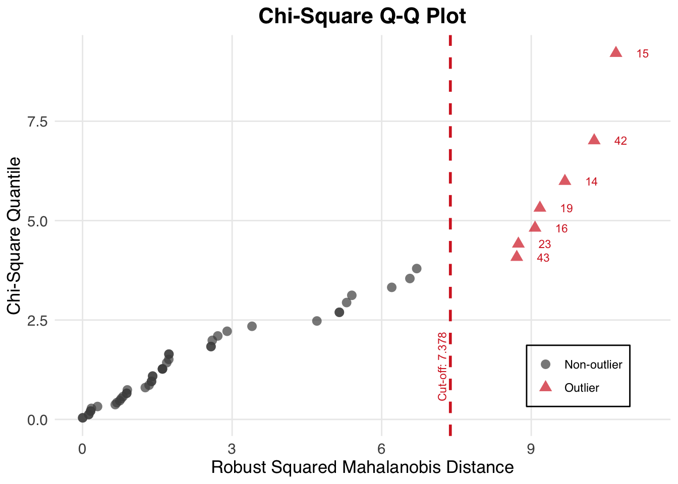

This Q–Q plot highlights points deviating from the theoretical chi-square line.

---

References

Korkmaz S, Goksuluk D, Zararsiz G. MVN: An R Package for Assessing Multivariate Normality. The R Journal. 2014;6(2):151–162. URL: https://journal.r-project.org/archive/2014-2/korkmaz-goksuluk-zararsiz.pdf